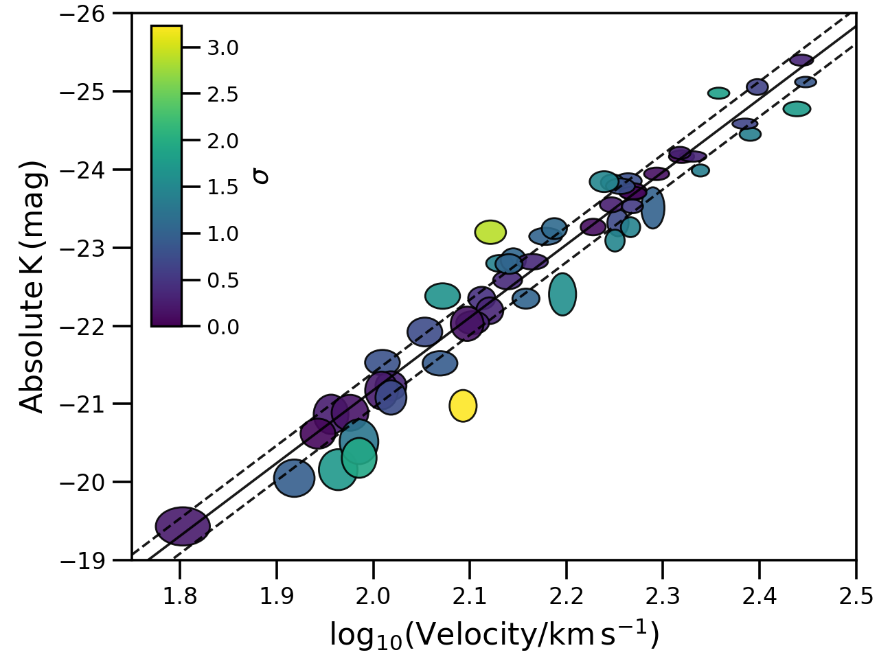
Tully-Fisher relation from Obreschkow & Meyer 2013

Run the fit and plot

from hyperfit.linfit import LinFit
from hyperfit.data import TFR

# Load the data
data = TFR()
hf = LinFit(data.xs, data.cov, weights=data.weights)

# Run an MCMC
bounds = ((-10.0, 10.0), (-1000.0, 1000.0), (1.0e-5, 500.0))
mcmc_samples, mcmc_lnlike = hf.emcee(bounds, verbose=True)
print(np.mean(mcmc_samples, axis=1), np.std(mcmc_samples, axis=1))

# Make the plot
data.plot(linfit=hf)

Returns

\[M_{K} \sim \mathcal{N}[\mu=(-9.2 \pm 0.4)\,\mathrm{log_{10}}V - (2.8 \pm 0.9)\, , \,\sigma=0.23 \pm 0.04]\]